Genetic information, variation and relationships between organisms (AQA AS Biology) PART 6 of 6 TOPICS
|
Investigating diversity:
Investigating diversity enables comparisons to be made:
- between different areas – comparing the biodiversity of one section of woodland with a similar type of woodland in another area to see which requires the most protection.
- in the same area at different times – comparing the biodiversity of a group of fields before and after hedgerows have been removed or replanted, or the biodiversity of a wood in two different seasons or at two different times of the day.
Genetic diversity within or between species can be made by comparing:
- the frequency of measurable or observable characteristics
- base sequence of DNA
- base sequence of mRNA
- amino acid sequence made in protein synthesis
Species richness is a number representing the different types of species in an area. The higher this number the more ‘rich’ an area is with species. The number of each individuals is not accounted for so only one individual of a species will have the same weight as a hundred individuals in another species.
Species evenness compares the size of a population where the individuals of species are accounted for.
Species diversity is directionally proportional to species richness and species evenness where if species richness and species evenness were to increase then species diversity increases.
Comparing biodiversity can be difficult as the following example shows:
| Species | Number of individuals in field 1 | Number of individuals in field 2 |
| Buttercup | 300 | 45 |
| Dandelion | 345 | 35 |
| Daisy | 355 | 920 |
| Total | 1000 | 1000 |
A conclusion can be drawn that field 1 has more species evenness than field 2 and so it has a greater biodiversity.
Index of diversity:
How to Calculate the Standard Deviation:
- Calculate the mean (x̅) of a set of data
- Subtract the mean from each point of data to determine (x-x̅). You’ll do this for each data point, so you’ll have multiple (x-x̅).
- Square each of the resulting numbers to determine (x-x̅)^2. As in step 2, you’ll do this for each data point, so you’ll have multiple (x-x̅)^2.
- Add the values from the previous step together to get ∑(x-x̅)^2. Now you should be working with a single value.
- Calculate (n-1) by subtracting 1 from your sample size. Your sample size is the total number of data points you collected.
- Divide the answer from step 4 by the answer from step 5
- Calculate the square root of your previous answer to determine the standard deviation.
- Be sure your standard deviation has the same number of units as your raw data, so you may need to round your answer.
- The standard deviation should have the same unit as the raw data you collected. For example, SD = +/- 0.5 cm.
The general formula for this however is:
NB: You are not required to work out standard deviations in the exam but in experiments it is needed to be learnt.
What does standard deviation show?
It shows how much the data is spread above and below the mean. A high standard deviation shows the data is more spread about the mean meaning it is less reliable however some will have a low standard deviation meaning the data is less spread out about the mean and is more reliable.
Statistical tests: Statistical tests include chi-squared, standard error and 95% confidence limits/t-test and Spearman’s rank correlation. Statistical tests are used to see if results are due to chance and if our null hypothesis (the theory which is most likely to be incorrect) is actually right. So how would you know which statistical test to use?
- Chi-squared: In a particular experiment certain values may be expected to be recorded and obtained in particular categories being investigated. These values are known as expected values. However other values may be obtained which are known as observed values. In this situation we need to use the chi-squared equation for this which is as follows:
Where O is observed and E is expected.
NB: You are not expected to work out chi squared in the exam however a demo will is given below. An example is in an A2 resource where chi-squared is covered again named ‘Genetics, populations, evolution and ecosystems 1’.
We have to come up with our null hypothesis which is: THERE IS NO SIGNIFICANT DIFFERENCE BETWEEN THE OBSERVED AND EXPECTED RESULTS.
It is best if you put your data for applying chi-squared in a table like the one below:
| Categories | O | E | O – E | (O – E)2 | (O – E)2/E | |||||||||
| Probability, p | ||||||||||||||
| Degrees of freedom | 0.25 (25%) | 0.20 (20%) | 0.15 (15%) | 0.10 (10%) | 0.05 (5%) | 0.02 (2%) | 0.01 (1%) | |||||||
| 1 | 1.32 | 1.64 | 2.07 | 2.71 | 3.84 | 5.41 | 6.63 | |||||||
| 2 | 2.77 | 3.22 | 3.79 | 4.61 | 5.99 | 7.82 | 9.21 | |||||||
| 3 | 4.11 | 4.64 | 5.32 | 6.25 | 7.81 | 9.84 | 11.34 | |||||||
| 4 | 5.39 | 5.99 | 6.74 | 7.78 | 9.49 | 11.67 | 13.28 | |||||||
| 5 | 6.63 | 7.29 | 8.12 | 9.24 | 11.07 | 13.39 | 15.09 | |||||||
NB: We should always use the column with the 0.05 or 5% probability highlighted in yellow as biologists always use this. The values in the table are known as critical values.
To know which degrees of freedom to use we must use the value that is 1 minus how many categories we have. You look at the corresponding critical value in the 5% probability column. If the chi-squared value is smaller than the critical value then we accept our null hypothesis saying that there is a 5% or higher probability that the results are due to chance and there is no significant difference between observed and expected values. NB: If our chi-squared value was greater than the critical value then we reject our null hypothesis and also say that there is a 5% or lower probability that the results are not due to chance and there is a significant difference between observed and expected value.
- Standard error and 95% confidence limits/t-test: If in an experiment you need to look at the differences between the means then we use the standard error and 95% confidence limits’ equation/t-test’s equation which is as follows:
Where SD is standard deviation and n is the number of results
NB: You are not expected to work out standard error and 95% confidence limits in the exam however a demo will is given below.
We have to come up with our null hypothesis which is: THERE IS NO DIFFERENCE BETWEEN THE TWO MEANS.
| Number of seeds that had germinated after 10 days | |||||||||||
| Seeds touching each other | Seeds placed 2 cm apart | ||||||||||
| 8 | 10 | 10 | 5 | 6 | 12 | 14 | 16 | 16 | 12 | 15 | 16 |
| 15 | 9 | 13 | 12 | 9 | 10 | 10 | 12 | 13 | 16 | 12 | 10 |
| 14 | 9 | 11 | 7 | 9 | 14 | 11 | 15 | 14 | 8 | 13 | 14 |
| 8 | 10 | 7 | 10 | 8 | 7 | 15 | 11 | 15 | 14 | 13 | 13 |
| 11 | 10 | 9 | 12 | 8 | 9 | 19 | 11 | 12 | 17 | 9 | 17 |
Some working out has to take place which is as follows:
SEEDS TOUCHING EACH OTHER
| Mean | (8+10+10+5+6+12+15+9+13+12+9+10+14+9+11+7+9+14+8+10+7+10+8+7+11+10+9+12+8+9)/30 = 9.73 |
| Σx2 | 64+100+100+25+36+144+225+81+169+144+81+100+196+81+121+49+81+196+64+100+49+ 100+64+49+121+100+81+144+64+81 = 3010 |
| (Σx)2 | 2922 = 85264 |
| Standard deviation | √(167.867/29) = 2.41 |
| Standard error | 2.41/√30 = 0.44 |
SEEDS PLACED 2CM APART
| Mean | (14+16+16+12+15+16+10+12+13+16+12+10+11+15+14+8+13+14+15+11+15+14+13+13+19+11+12+17+9+17)/30 = 13.43 |
| Σx2 | 196+256+256+144+225+256+100+144+169+256+144+100+121+225+196+64+169+196+225+121+225+196+169+169+361
121+144+289+81+289 = 5607 |
| (Σx)2 | 4032 = 162409 |
| Standard deviation | √(193.367/29) = 2.58 |
| Standard error | 2.58/√30 = 0.47 |
The 95% confidence limits is double the standard error above and below the mean which is as follows continued from the example shown above:
SEEDS TOUCHING EACH OTHER
| Upper limit | (2 x 0.44) + 9.73 = 10.61 |
| Lower limit | 9.73 – (2 x 0.44) = 8.85 |
SEEDS PLACED 2CM APART
| Upper limit | (2 x 0.47) + 13.43 = 14.37 |
| Lower limit | 13.43 – (2 x 0.47) = 12.49 |
These limits are represented in the graph below:
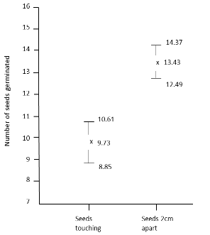
If the 95% confidence limits do overlap then we accept the null hypothesis saying there is 5% or higher probability that the difference between the two means is due to chance alone. NB: If the 95% confidence limits do not overlap then we reject the null hypothesis saying there is less than 5% probability that the difference between the means values is not due to chance. In this case we reject.
- Spearman’s rank correlation: After an experiment, if you want to see if there is any association of two sets of data then you would use this test.
Where D is the rank and n is the number of observations
NB: The Spearman’s rank correlation (Rs) value will be between either -1 and 0 or 0 and 1.
NB: You are not expected to work out Spearman’s rank correlation in the exam however a demo will is given below.
NB: The difference in rank (D) squared must add up to 6.5.
We have to come up with our null hypothesis which is: THERE IS NO ASSOCIATION BETWEEN THE TWO SETS OF RESULTS.
| Mass of egg / g | 1.37 | 1.49 | 1.56 | 1.70 | 1.72 | 1.79 | 1.93 |
| Mass of chick on hatching / g | 0.99 | 0.99 | 1.18 | 1.16 | 1.17 | 1.27 | 1.75 |
The first step is to start ranking the mass of egg or the mass of the chick from smallest to biggest or vice versa. NB: This is because if the two were ranked each mass of egg or chick would not be corresponding to the other value in the other set of data. Also if two values have the rank then you divide the rank they share by two, e.g. For the mass of chick there are two chicks that have a mass of 0.99. As this value is the smallest out of all the other masses of chicks it has a rank of 1. Divide 1 by two to get 0.5. The ranks are shown in the table below:
| Individual number | Egg mass / g | Rank | Chick mass / g | Rank | Difference in rank (D) | D2 |
| 1 | 1.37 | 1 | 0.99 | 1.5 | 0.5 | 0.25 |
| 2 | 1.49 | 2 | 0.99 | 1.5 | 0.5 | 0.25 |
| 3 | 1.56 | 3 | 1.18 | 5 | 2 | 4 |
| 4 | 1.70 | 4 | 1.16 | 3 | 1 | 1 |
| 5 | 1.72 | 5 | 1.17 | 4 | 1 | 1 |
| 6 | 1.79 | 6 | 1.27 | 6 | 0 | 0 |
| 7 | 1.93 | 7 | 1.75 | 7 | 0 | 0 |
In the table above the D2 values add up to 6.5. Work out the Rs value which comes to be 0.884 when n is substituted for 7 and ƩD2 is substituted for 6.5. NB: A positive Rs value shows it is more likely that there is an association. A negative Rs value shows it is more likely that there is no association. However an Rs value of zero shows that there is definitely no association. Then compare your Rs value with the critical values below:
| Number of pairs of measurements | Critical value |
| 5 | 1.00 |
| 6 | 0.89 |
| 7 | 0.79 |
| 8 | 0.74 |
| 9 | 0.68 |
| 10 | 0.65 |
| 12 | 0.59 |
| 14 | 0.54 |
| 16 | 0.51 |
| 18 | 0.48 |
As we have 7 pairs of data we have to look at the corresponding critical value to the number of pairs which in this case is 0.79 highlighted in yellow. Our Rs of 0.884 is bigger than the critical value and so we reject our null hypothesis by saying there is a 5% or lower probability that the results are not due to chance and there is a significant correlation between the two sets of data. NB: If our Rs value is smaller than the critical value we accept our null hypothesis by saying there is a 5% or higher probability that the results are due to chance and that there is no significant correlation between the two sets of data.